The Second National Data Science Bowl, a data science competition where the goal was to automatically determine cardiac volumes from MRI scans, has just ended. We participated with a team of 4 members from the Data Science lab at Ghent University in Belgium and finished 2nd of 192 competing teams.

The team kunsthart (artificial heart in English) consisted of Ira Korshunova, Jeroen Burms, Jonas Degrave (@317070), 3 PhD students, and professor Joni Dambre. It’s also a follow-up of last year’s team Deep Sea, which finished in first place for the First National Data Science Bowl.

Introduction

The problem

The goal of this year’s Data Science Bowl was to estimate minimum (end-systolic) and maximum (end-diastolic) volumes of the left ventricle from a set of MRI-images taken over one heartbeat. These volumes are used by practitioners to compute an ejection fraction: fraction of outbound blood pumped from the heart with each heartbeat. This measurement can predict a wide range of cardiac problems. For a skilled cardiologist analysis of MRI scans can take up to 20 minutes, therefore, making this process automatic is obviously useful.

Unlike the previous Data Science Bowl, which had very clean and voluminous data set, this year’s competition required a lot more focus on dealing with inconsistencies in the way the very limited number of data points were gathered. As a result, most of our efforts went to trying out different ways to preprocess and combine the different data sources.

The data

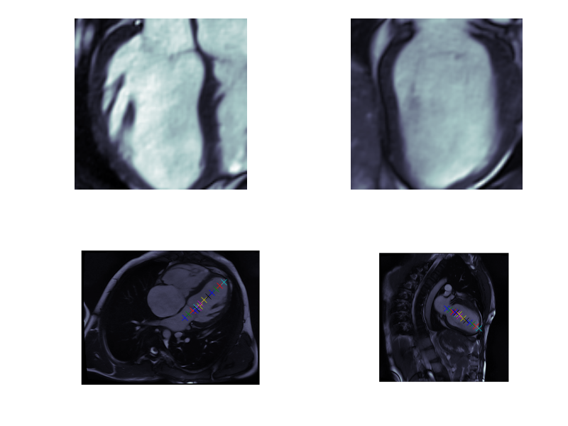
The dataset consisted of over a thousand patients. For each patient, we were given a number of 30-frame MRI videos in the DICOM format, showing the heart during a single cardiac cycle (i.e. a single heartbeat). These videos were taken in different planes including the multiple short-axis views (SAX), a 2-chamber view (2CH), and a 4-chamber view (4CH). The SAX views, whose planes are perpendicular to the long axis of the left ventricle, form a series of slices that (ideally) cover the entire heart. The number of SAX slices ranged from 1 to 23. Typically, the region of interest (ROI) is only a small part of the entire image. Below you can find a few of SAX slices and 2CH, 4CH views from one of the patients. Red circles on the SAX images indicate the center of ROI (later we will explain later how to found it), for 2CH and 4CH they specify the location of SAX slices projected on the corresponding view.

sax_5

sax_9

sax_10

sax_11

sax_12

sax_15

2CH

4CH

The DICOM files also contained a bunch of metadata. Some of these metadata fields were absolutely invaluable to us. Examples include the PixelSpacing (which specifies the resolution of the image) and the ImageOrientation. The metadata also specified the patient’s age and sex.

For each patient in the train set, two labels were provided: the systolic volume and the diastolic volume. From what we gathered (link), these were obtained by the cardiologists by manually performing a segmentation on the SAX slices, and feeding these segmentations to a program that in turn computed the minimal and maximal heart chamber volumes out of these. The cardiologists didn’t use the 2CH or 4CH images to estimate the volumes, but these proved to be very useful to us nevertheless.

Although combining these multiple different data sources can be challenging, we found the main challenge in dealing with this data set to be the handling of the inconsistencies in the data. Some obvious examples include the 4CH slice not being provided for some patients, that one patient whose SAX slice videos consisted of less than 30 frames, or the couple of patients who only had a handful of SAX slices, not even covering the entire heart. More subtle examples include patients whose series of SAX slices were taken in very weird locations.

The evaluation

Given a patient’s data, we were asked to output a cumulative distribution function over the volume, ranging from 0 to 599 mL, for both systole and diastole. The models were scored by a Continuous Ranked Probability Score (CRPS) error metric, which computes the average squared distance between the predicted CDF and a Heaviside step function representing the real volume.

An additional interesting novelty of this competition was the two stage process. In the first stage, we were given a training set of 500 patients with a public test set of 200 patients. In the final week we were required to submit our model and afterwards the organizers released the test data of 440 patients and labels for those 200 patients from the public test set. We think the goal was to compensate for the small dataset and prevent people from optimizing against the test set through visual inspection of every part of their algorithm.

The solution: traditional image processing, convnets, and dealing with outliers

In our solution, we combined traditional image processing approaches, which find the region of interest (ROI) in each slice, with convolutional neural networks, which perform the mapping from the extracted image patches to the predicted volumes. Given the very limited number of training samples, we tried combat overfitting by restricting our models to combine the different data sources in predefined ways, as opposed to having them learn how to do the aggregation. Finally, a key insight that led to our approach was that it would have been a bad idea to try and make one model that is capable of processing every single patient, given the large amount of inconsistencies in the data. Instead, we tried to make models that were able to, for example, assume that SAX slices nicely ranged from one end of the heart to the other, and let model who were robust to this not being the case handle the outliers. Of course, this approach also makes it vital to recognise which model apply to which patients.

In what follows, we discuss exactly the various types of pre-processing we did in order to make our models robust against some of the problems in the data, and make the information cleaner and more chewable for the models.

Pre-processing

The provided images have varying sizes and resolutions, and do not only show the heart, but the entire torso of the patient. Our preprocessing pipeline made the images ready to be fed to a convolutional network by going through the following steps:

• applying a zoom factor such that all images have the same resolution in millimeters.
• finding the region of interest (ROI) and extracting a patch centered around it.
• data augmentation

To find the correct zooming factor, we made use of the “PixelSpacing” metadata field, which specifies the image resolution. Next, to find the region of interest, we developed two methods, one based on the relative positioning of the 2CH, 4CH and SAX slices, and one based on image segmentation techniques.

Detecting the Region Of Interest through metadata

One approach to find the region of interest is to intersect the different images in 3D space. If you assume the left ventricle to be visible in each image (an assumption which is usually, but sadly not always, correct), then the points where the 2CH, 4CH and one of the SAX slices cross, should be inside the heart chamber we are looking for.

In this way, we can obtain a single point in each SAX slice, which we use as the center for the region of interest. In the 2CH and 4CH slices, we obtain multiple points, which (usually) nicely range from the bottom to the top of the left ventricle. As a result we can cut out nice squares which closely encompass the left ventricle.

Detecting the Region Of Interest through image segmentation techniques

We used classical computer vision techniques to find the left ventricle in the SAX slices. For each patient, the center and width of the ROI were determined by combining the information of all the SAX slices provided. Fig. 3 (left image) shows an example of the result.

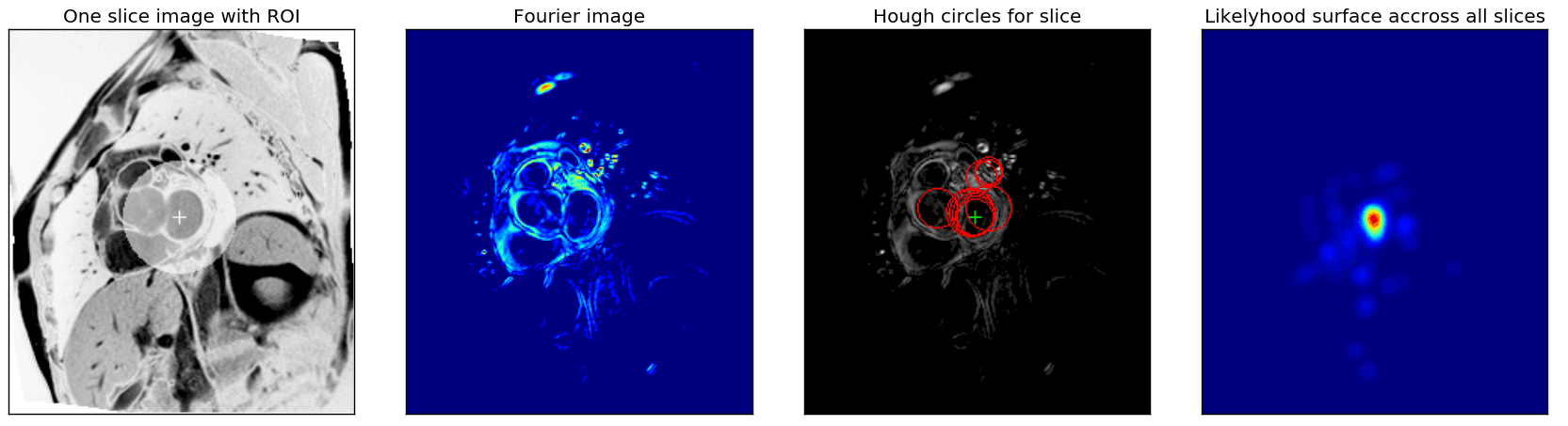
First, as was suggested in the Fourier based tutorial, we exploit the fact that each slice sequence captures one heartbeat and use fourier analyses to extract an image that captures the maximal activity at the corresponding heartbeat frequency (Fig. 3, second image).

From these Fourier images, we then extracted the center of the left ventricle by combining the Hough circle transform with a custom kernel-based majority voting approach across all SAX slices. First, for each fourier image (resulting from a single sax slice), the N highest scoring Hough circles for a range of radii were found, and from all of those, the M highest scoring ones were retained. N, M and the range of radii are metaparameters that severely affect the robustness of the ROI detected and were optimised manually. The third image in Fig. 3 shows an example of the M best circles for one slice.

Finally, a ‘likelihood surface’ (rightmost image in Fig. 3) was obtained by combining the centers and scores of the selected circles for all slices. Each circle center was used as the center for a Gaussian kernel, which was scaled with the circle score, and all these kernels were added. The maximum across this surface was selected as the center of the ROI. The width and height of the bounding box of all circles with centers within a maximal distance (another hyperparameter) of the ROI center were used as bounds for the ROI or to create an ellipsoidal mask as shown in the figure.

Besides manual parameter optimisation, the algorithm was made robust by expressing all distance-related hyperparameters relatively to the “PixelSpacing” metadata field

Given these ROIs in the SAX slices, we were able to find the ROIs in the 2CH and 4CH slices by projecting the SAX ROI centers onto the 2CH and 4CH planes.

Deep learning

We used convolutional neural networks to learn a mapping from the extracted image patches to the predicted systolic and diastolic volumes. During the competition, we played around a lot with both minor and major architectural changes. In this section, we’ll explain what our mainstream models looked like, and how we trained them, as well as going over some of the alternatives we tried out.

Architectures

Our base architecture for most of our models was based on VGG-16. It seemed to work pretty well on this dataset, despite probably having too many parameters for the small number of patients. We tried to mitigate the overfitting in various ways (see this section).

As we already mentioned, we trained different models which can deal with different kinds of patients. There are roughly four very different kinds of models we trained: single slice models, patient models, 2CH models and 4CH models.

Single slice models

Single slice models are models that take a single SAX slice as an input, and try to predict the systolic and diastolic volumes directly from it. The 30 frames were fed to the network as 30 different input channels. The systolic and diastolic networks shared the convolutional layers, but the dense layers were separated. The output of the network could be either a 600-way softmax (followed by a cumulative sum), or the mean and standard deviation of a Gaussian (followed by a layer computing the cdf of the Gaussian).

Although these models obviously have way too little information to make a decent estimation about the volume of the heart, they benefitted hugely from test-time augmentation (TTA). During TTA, the same single slice model is fed the different SAX slices (with different augmentations) of the same patient, and the outputs are averaged. Although this way of aggregating information over SAX slices is suboptimal, it proved to be very robust to the relative positioning of the SAX slices, and is as such applicable to all patients.

Our single best single slice model achieved a local validation score of 0.0157 (after TTA), which was a reliable estimate for the public leaderboard score for these models. It had the following architecture for both systole and diastole:

2CH and 4CH models

2CH and 4CH models look a the ROI in the 2CH and 4CH slices respectively. These models have a much more global view on the left ventricle of the heart than the single slice models. We used a similar architecture for these. Just like the single slice models, the 2CH models also have the advantage of being applicable to every patient. Not every patient had a 4CH slice provided. We used the same VGG-inspired architecture for these models. Individually, they achieved a similar validation score (0.0156) as was achieved by averaging over multiple sax slices. By ensembling only single slice, 2CH and 4CH models, we were able to achieve a score of 0.0131 on the public leaderboard.

Patient models

As opposed to single slice models, patient models try to make predictions based on the entire stack of (up to 22) SAX slices. In our first approaches to these models, we tried to process each slice separately using a VGG-like single slice network, followed by feeding the results to an overarching RNN or LSTM in an ordered fashion. However, these models tended to overfit quite badly, probably because of the limited amount of training samples.

Our solution to this problem consists of an innovative way to merge predictions from multiple slices. Instead of having the network learn how to compute the volume based on the results of the individual slices, we designed a layer which combines the areas of consecutive cross-sections of the heart using a truncated cone approximation.

Since these formulas are derivable, we can still train models using this type of aggregation end-to-end. Using this improved our results and training speed massively. Adding a priori information into your model architecture is always a good idea.

One downside of this approach was that these models assume that the SAX slices nicely range from one end of the heart to the other. This was trivially not true for patients with very few (< 6) slices, but it was harder to detect automatically for some other outlier cases as in figure below, where something is wrong with the images or the ROI algorithm fails.

sax_12

sax_15

sax_17

sax_36

sax_37

sax_41

2CH

4CH

Ordering the SAX slices and finding the distance between them was achieved through looking at the SliceLocation metadata fields, but this field was not very reliable in finding the distance between slices, neither was the SliceThickness. We looked for the two slices that were furthest apart, drew a line between them, and projected every other slice onto this line. This way, we estimated the distance between two slices ourselves.

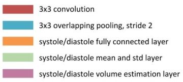
Our best single model achieved a local validation score of 0.0105 using this approach, although this is no longer a very good leaderboard estimations, since our local validation set contained relatively few outliers compared to the public leaderboard in the first round. It had the following architecture for both systole and diastole:

Layer Type	Size	Output shape
Input layer		(8, 25, 30, 64, 64)*
Convolution	128 filters of 3x3	(8, 25, 128, 64, 64)
Convolution	128 filters of 3x3	(8, 25, 128, 64, 64)
Max pooling		(8, 25, 128, 32, 32)
Convolution	128 filters of 3x3	(8, 25, 128, 32, 32)
Convolution	128 filters of 3x3	(8, 25, 128, 32, 32)
Max pooling		(8, 25, 128, 16, 16)
Convolution	256 filters of 3x3	(8, 25, 256, 16, 16)
Convolution	256 filters of 3x3	(8, 25, 256, 16, 16)
Convolution	256 filters of 3x3	(8, 25, 256, 16, 16)
Max pooling		(8, 25, 256, 8, 8)
Convolution	512 filters of 3x3	(8, 25, 512, 8, 8)
Convolution	512 filters of 3x3	(8, 25, 512, 8, 8)
Convolution	512 filters of 3x3	(8, 25, 512, 8, 8)
Max pooling		(8, 25, 512, 4, 4)
Convolution	512 filters of 3x3	(8, 25, 512, 4, 4)
Convolution	512 filters of 3x3	(8, 25, 512, 4, 4)
Convolution	512 filters of 3x3	(8, 25, 512, 4, 4)
Max pooling		(8, 25, 512, 2, 2)
Fully connected	1024 units	(8, 25, 1024)
Fully connected	1024 units	(8, 25, 1024)
Fully connected	2 units (mu and sigma)	(8, 25, 2)
Volume estimation		(8, 2)
Gaussian CDF		(8, 600)

* The first dimension is the batch size, i.e. the number of patients, the second dimension is the number of slices. If a patient had fewer slices, we padded the input and omitted the extra slices in the volume estimation.

Oftentimes, we did not train patient models from scratch. We found that initializing patient models with single slice models helps against overfitting, and severely reduces training time of the patient model.

Alternative architectures

The architectures we described above were the ones that worked the best for us. To deversify our models, some of the good things we tried include:

• Processing each frame separately, and taking the minimum and maximum at some point in the network to compute systole and diastole. Although this worked, these models never achieved the same results, were more finicky and had to train longer.
• Having the CNN output a segmentation mask, in which each pixel represents the probability that it is part of the left ventricle. There are no longer any max-pooling layers, and the dense layers are replaced by a simple integration over the outputted mask. Again, this worked to a certain extent, but never achieved comparable results. Furthermore, these networks eat a lot of GPU memory, and as such required some tricks to fit on them. sharing some of the dense layers between the systole and diastole networks as well
• using discs to approximate the volume, instead of truncated cones
• cyclic rolling layers
• leaky RELUs
• maxout units

Some of the things we tried, but didn’t work:

• A variant of highway networks and residual networks. These failed to perform very well, probably due to the small dataset, whereas these networks mostly shine in very big datasets.
• Sharing some of the dense layers between the systole and diastole networks as well. This didn’t improve our results.
• Training convolutional layers on the sunny dataset as well

Training

Error function

At the start of the competition, we experimented with various error functions. We tried using log-losses for a classification approach (weighted with the distance from the correct value), and tried an L1- and L2-error on a regression task as well. In the end, we found optimising CRPS directly to work best, although we had to tweak the optimizer in order to keep it stable in the first few steps of the optimization process.

Training algorithm

To train the parameters of our models, we used the Adam update rule (Kingma and Ba). We found this was necessary in order to optimize CRPS directly.

Initialization

We initialised all filters and dense layers orthogonally (Saxe et al.). Biases were initialized to small positive values to have more gradients at the lower layer in the beginning of the optimization. At the Gaussian output layers, we initialized the biases for mu and sigma such that initial predictions of the untrained network would fall in a sensible range. The exact values differed from model to model though.

Regularization

Since we had a low number of patients, we needed considerable regularization to prevent our models from overfitting. Our main approach was to augment the data (as described in the following section), and to add considerable amount of dropout (p = 0.5).

Data augmentation

As always when using deep learning on a problem with few training examples, we used tons of data augmentation. In this case, some special precautions need to be made. There are only a couple of transformations which preserve surface area (namely when the projection surface has a zero gauss curvature). In terms of affine transformations, this means only skewing, rotation and translation is allowed. Of these, the first two are the most interesting for a convnet, since it is inherently robust against translations.

Despite this, we also added zoom, but we had to also correct our volume labels when doing so! This means that you change the distribution of heart sizes found in the dataset, so it needs to be applied separately and carefully. However, some heart sizes are not found in the dataset, so this augmentation also helped to smooth out the found predictions, especially when we use a more classification-like approach.

Another augmentation here came in the form of shifting the images over the time axis. While systole was often found in the beginning of a sequence, this was not always the case. Augmenting this, by rolling the image tensor over the time axis, made the resulting model more robust against this noise in the dataset, while providing even more augmentation of our data.

These data augmentations were applied during the training phase to increase the number of training examples. We also applied the augmentations during the testing phase, and averaged predictions across the augmented versions of the same data sample. This should make our algorithm more robust against outliers, and helps estimating the uncertainty of the prediction. We used quasi-random sampling to sample the augmentation parameters, since what you are effectively doing is integrating over a space in your augmentation parameters, and integrating is more effective when using quasi-random than pseudo-random. This is true both during training and testing.

Validation

Since the trainset was already quite small, we kept the validation set small as well (1 out of 6). As a result, our validation score would be quite noisy, but then again, the preliminary and final leaderboards would be as well (respectively 200 and 440 patients, versus our own set of 83 patients).

Despite this, our validation score remained pretty close to the leaderboard score. Also, in cases where it didn’t, it helped us identify issues in our models, namely problematic cases in the test set which were not represented in our validation set. We noticed for instance that quite some of our patient models had problems with patients with too few SAX slices (< 5).

Selectively train and predict

By looking more closely at the validation scores, we observed that most of the accumulated error was obtained by wrongly predicting only a couple of such outlier cases. At some point, being able to handle only a handful of these meant the difference between a leaderboard score of 0.0148 and 0.0132!

To mitigate such issues, we set up our framework such that each individual model could choose not to train on or predict a certain patient. For instance, models on patients’ SAX slices could choose not to predict patients with too few SAX slices, models which use the 4CH slice would not predict for patients who don’t have this slice. We extended this idea further by developing expert models, which only trained and predicted for patients with either a small or a big heart (as determined by the ROI detection step). Further down the pipeline, our ensembling scripts would then take these non-predictions into account.

Ensembling and dealing with outliers

We ended up creating about 250 models throughout the competition. However, we knew that some of these models were not very robust to certain outliers or patients whose ROI we could not accurately detect. We came up with two different ensembling strategies that would deal with these kind of issues.

Our first ensembling technique followed the following steps:

1. For each patient, we select the best way to average over the test time augmentations. Slice models often preferred a geometric averaging of distributions (since not all slices of a patient contain enough information to predict volume) whereas in general arithmetic averaging worked better for patient models.
2. We average over the models by calculating each prediction’s KL-divergence from the average distribution, and the cross entropy of each single sample of the distribution. This means models which are further away from the average distribution get more weight (since they are more certain). It also means samples of the distribution closer to the median-value of 0.5 get more weight. Each model also receives a model-specific weight, which is determined by optimizing these weights over the validation set.
3. Since not all models predict all patients, it is possible for a model in the ensemble to not predict a certain patient. In this case, a new ensemble without these models is optimized, especially for this single patient. The method to do this is described in step 2.
4. This ensemble is then used on every patient on the test-set. However, when a certain model’s average prediction disagrees too much with the average prediction of all models, the model is thrown out of the ensemble, and a new ensemble is optimized for this patient, as described in step 2. This meant that about ~75% of all patients received a new, personalized ensemble.

Especially because of this last step, this way of ensembling should be able to remove models from the ensemble that can’t handle a certain outlier very wel.

Our second way of ensembling involves comparing an ensemble that is suboptimal, but robust to outliers, to an ensemble that is not robust to them. This approach is especially interesting, since it does not need a validation set to predict the test patients. It follows the following steps:

1. Again, for each patient, we select the best way to average over the test time augmentations again.
2. We combine the models by using a weighted average on the predictions, with the weights summing to one. These weights are determined by optimising them on the validation set. In case not all models provide a prediction for a certain patient, it is dropped for that patient and the weights of the other models are rescaled such that they again sum to one. This ensemble is not robust to outliers, since it contains patient models.
3. We combine all 2CH, 4CH and slice models in a similar fashion. This ensemble is robust to outliers, but only contains less accurate models.
4. We detect outliers by finding the patients where the two ensembles disagree the most. We measure disagreement using CRPS. If the CRPS exceeds a certain threshold for a patient, we assume it to be an outlier. We chose this threshold to be 0.02.
5. We retrain the weights for the first ensemble, but omit the outliers from the validation set. We choose this ensemble to generate predictions for most of the patients, but choose the robust ensemble for the outliers.

Following this approach, we detected three outliers in the test set during phase one of the competition. Closer inspection revealed that for all of them either our ROI detection failed, or the SAX slices were not nicely distributed across the heart. Both ways of ensembling achieved similar scores on the public leaderboard. (0.0110)

Second round submissions

For the second round of the competition, we were allowed to retrain our models on the new labels. We were also allowed to plan two submissions. Of course, it was impossible to retrain all of our models during this single week. For this reason, we chose to only train our 44 best models, according to our ensembling scripts. These are not necessarily the models which achieve the best individual scores, but rather the models that achieve decent scores but are nonetheless very different architectures.

For our first submission, we again split of a validation set, and retrain all of the models on the remainder of the train set. The resulting models were combined using our first ensembling script. This submission can be considered a rather safe one, since if something goes wrong with one of the models for whatever reason, the merging script will detect it by looking at the validation scores, and omit the model from the ensemble.

For our second submission, we trained our models on the entire training set (i.e. there was no validation split). We assembled them using using the second ensembling method. Since we had no validation set to optimise the weights of the ensemble on, we computed the weights by training an ensemble on the models we trained with a validation split, and transferred them over. This submission could be considered as a shot at first place, but could as well fail if some model goes wrong on a single patient.

Software and hardware

We used Lasagne, Python, Numpy and Theano to implement our solution, in combination with the cuDNN library. We also used PyCUDA for a few custom kernels.

We made use of scikit-image for pre-processing and augmentation, and ghalton for quasi-random number generation.

We trained our models on the NVIDIA GPUs that we have in the lab, which include GTX TITAN X, GTX 980, GTX 680 and Tesla K40 cards. We would like to thank Frederick Godin and Elias Vansteenkiste for lending us a few extra GPUs in the last week of the competition.

Rant on the competition

Overall, we disliked the current competition compared to other previous competitions we have done on Kaggle.

First of all, we dislike the two round method, where you only get the final test data in the final week, and were not allowed to change your model in that week. We reckon it was chosen because of the limited amount of data, such that nobody can visually check every step of their algorithm on the test set (and thus almost hand-label the test set). However, it leaves a lot to desire: we know Kaggle cannot check the models at the end of the competition, therefore, the ranking after third place is effectively useless. The forums prove that there are people still changing their models after having received the test data, and while they discard any monetary reward upfront, they do still share the leaderboard with people who played the competition ‘honestly’. It is not to hard to do visual checking on most parts of the algorithm discussed earlier, especially the finding of the ROI can be optimized until it is perfect on the entire set, including the test set.

A second problem with the two round method is that you need to be available in that final week, and spend considerable effort in that week in order to compete. Not only that, if the model needs to evaluate in one week, it gives additional benefit to people with (expensive) hardware, such as ourselves. Other Kaggle competitions are more open in comparison.

We also disliked the very noisy and bugged dataset. As we joined this competition mainly out of academic interest, as a way to test the new algorithms on a dataset, this dirty data was uninteresting. It posed some technical challenges, which we are sure is very relevant for the real world data engineer, but we feel like in this case it went a little over the top. Also the fact that the ground truth was hand-labeled with a noisy (and varying!) method made sure that the achievable accuracy would be limited and dependent on which patients were in the final test set. This post is written before we know the final leaderboard, but we wouldn’t be surprised if this leaderboard turns out to be considerably different from the previous leaderboard. We don’t feel as if the task is not interesting or challenging, rather that the threshold to load and preprocess the data was considerable, and limited the amount of time which could be spent on actual machine learning algorithms.

Both the fact that the dataset was small and noisy, will probably have lead to many people optimizing using hand-labels. We feel this kind of defeats the point of such a competition, and in the end, regret not having done it ourselves.

Conclusion and TL;DR

We learned a lot from this competition and are happy with our results. We tried out different ways to preprocess data and combine information from different data sources, and learned a lot in this aspect.

However, we feel that there is still a lot of room for improvement. For example, we observed that most of our error still hails from a select group of patients. These include the ones for which our ROI extraction fails. In hindsight, hand-labeling the training data and training a network to do the ROI extraction would probably be a better approach, but we wanted to sidestep doing a lot of this kind of manual effort as much as possible. In the end, labeling the data would probably have been less time intensive anyways, albeit a lot more mind-numbing as well.

We reckon we will do more Kaggle competitions in the future, albeit that we will stay away from future two round, dirty data, small dataset competitions.

---

• ← Previous Post
• Next Post →